High-pass cutoffs that distort slow ERPs
Symptom. Artifactual early components; attenuated late components.
Symptom
A “component” appears or vanishes when the high-pass cutoff changes. Typical forms: a late, slow positivity (P3, CNV, late positive potential) is smaller than expected or absent; an early negativity of opposite sign to a later component appears before it (an apparent N1 or “anticipatory” negativity that no one predicted); a pre-stimulus baseline that slopes; a condition difference that shrinks, grows or reverses across cutoffs in a multiverse.
Cause
Slow ERP components have most of their energy at low frequencies. A high-pass filter removes that energy, and because the standard offline filter is zero-phase, the removed energy is redistributed symmetrically in time: a large positive deflection is accompanied by negative deflections before and after it that were not in the data. The higher the cutoff (and the sharper the filter), the larger and longer these artifacts. A cutoff that is harmless for a brief early component such as P1 can halve a P3 and invent an N1-like deflection before it.
Detect
- Filter a single trace containing a known slow transient (the sandbox’s electrode pop, or a simulated boxcar of the component’s duration) with your chosen high-pass and look at what appears on either side.
- Compute the ERP at several high-pass cutoffs (0.01, 0.1, 0.5, 1 Hz) and plot them together; an amplitude that falls steadily with cutoff, or a deflection that grows with cutoff, is a filter product.
- Check the impulse and step response of the filter: any overshoot in the step response will appear around every slow component.
- Ask whether the “component” has a plausible topography and latency of its own, or simply mirrors the later component with opposite sign.
Fix
- Use a conservative high-pass for ERPs — on the order of 0.1 Hz or lower — with a gentle transition band, and state the cutoff, filter type, order or length, and direction (zero-phase or causal) in the methods.
- Treat the cutoff as an analysis choice to be justified, not a default: filter as little as the data allow and remove drift by other means where possible (good recording practice, baseline correction, or regression-based approaches).
- Never choose the cutoff by which one makes the effect look best; if several cutoffs are defensible, report the effect across them (L6.4).
- Filter continuous data before epoching; see pf-filter-epoched-data.
Example
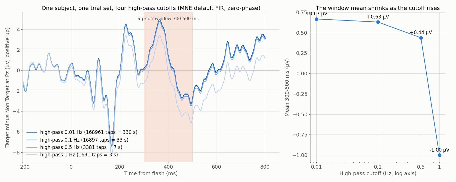
ds-brain-invaders bi2014a subject 1 (via moabb), Pz: 1135 of 1188 flashes kept (189 Target, 946 Non-Target; the same trials at every cutoff), common 30 Hz low-pass, high-pass at 0.01 / 0.1 / 0.5 / 1 Hz with MNE’s default FIR, epochs −0.2 to 0.8 s, baseline −0.2 to 0 s, recording reference kept — the pipeline of nb-1-5-filters. The 300–500 ms window means are 0.67, 0.63, 0.44 and −1.00 µV, the numbers the L1.5 exercise asks for. Generated by data/scripts/make_figures.py (CC BY 4.0; label_source: algorithmic). ERP CORE remains the intended source once §13 item 22 is resolved.