Removing brain components that carry the effect
Symptom. Effect shrinks after "cleaning"; components with alpha or posterior topography removed.
1 claim on this page is unverified. TODO(confirm) marks a specific statement the author has not yet checked against a
primary source. Everything else on this page has been reviewed. Treat a marked claim as
provisional and go to the cited source rather than quoting the sentence.
Symptom
The effect is smaller after cleaning than before it, or disappears entirely. The number of components removed varies wildly from subject to subject — two for one participant, nineteen for the next. The removed list includes components with smooth, dipolar topographies and physiological spectra, or a posterior component with a clear alpha peak. Cleaned data has visibly less variance in the band the study is about. With ASR rather than ICA the symptom is quieter: the data simply looks clean, high-amplitude transients are gone, and the effect is smaller.
Cause
Every component you remove is subtracted from the data. If it carried brain activity, so is your effect.
Three routes lead there:
- Removing a class because of its name. “Alpha is noise” is true for some analyses and false for the study measuring alpha. A posterior component with a 10 Hz peak and a dipolar occipital map is the best candidate for a real generator in the whole decomposition.
- Removing the “other” class. In the ICLabel scheme, other means the classifier cannot tell. Treating it as a synonym for artifact removes precisely the components about which there is least evidence.
- Removing on one view. A component that looks muscle-like in its spectrum may be a brain component in a recording with broadband noise; a component with a large deflection in its time course may be a genuine evoked response. Classification needs convergent evidence from topography, time course, spectrum and ERP image.
ASR’s version of the mechanism is structural rather than a labelling error. It removes, per short window, any subspace whose variance exceeds a calibration statistic — which is a description of high-amplitude, transient, non-stationary activity, and therefore of bursts, epileptiform transients and large evoked responses as well as of artifact. Because ASR reconstructs the removed subspace from the retained one instead of deleting it, the output looks continuous and full-rank, and there is no list of removed components to inspect.
Detect
- Compute the effect with and without the cleaning step. This is the decisive test, and it is cheap. A cleaning step that moves the effect is a step that needs justifying.
- Count removed components per subject and look at the distribution. Large variance across subjects means the criterion is not the same criterion each time.
- Review the removed set: any component with a smooth dipolar topography, a 1/f-like spectrum with a physiological peak, or a consistent event-locked deflection in its ERP image is a component to argue about before removing.
- Compare the spectrum before and after cleaning. A band that lost power without a corresponding artifact in the removed components is a warning.
- Check the rank of the cleaned data against what the pipeline log says it should be.
- For ASR: vary the cutoff over a range and plot the effect against it. A result that depends strongly on the cutoff is a result about the cutoff.
Fix
- Decide the removal policy before you look at the effect: which classes are removed, on what evidence, and what the upper limit on the number removed is. Apply it identically to every subject.
- For each removed component, record the class, the evidence from each view, and the classifier probability if available, in the QC report (L2.8). If the justification needs “probably” more than once, keep the component and say so.
- Use the classifier as a second opinion and a triage, not an oracle: agreement settles a component, disagreement marks it for inspection.
- Prefer removing fewer components and reporting the residual artifact to removing more and reporting nothing.
- With ASR, report the cutoff and the calibration segment, and show the analysis at a second cutoff. Where the analysis targets high-amplitude transient activity, prefer a method whose removals can be listed.
- Report both the cleaned and the uncleaned result whenever they differ materially. Being unable to do so is itself a finding about the pipeline.
Example
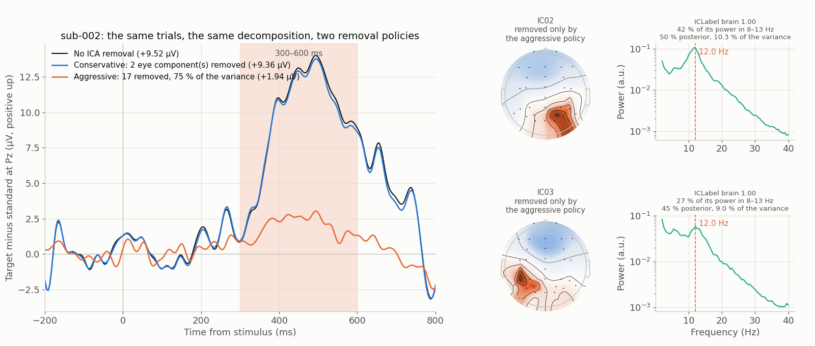
TODO(confirm): caption and numbers, once data/scripts/make_figures_p2.py has written /figures/pitfalls/pf-overcleaning-ica.png and its sidecar — including the subject, the two removal policies, the number of components removed under each, and the window-mean amplitudes. The figure is generated from the ds-erpcore P3 data that w-ica-component-gallery and w-threshold-tuner also draw on (CC BY 4.0; derived: filtered, decomposed, epoched). The description above states what the mechanism requires the figure to show; the sidecar’s own alt and caption are the authority once it exists.