Mass univariate tests without correction
Symptom. Significant blobs everywhere.
1 claim on this page is unverified. TODO(confirm) marks a specific statement the author has not yet checked against a
primary source. Everything else on this page has been reviewed. Treat a marked claim as
provisional and go to the cited source rather than quoting the sentence.
Symptom
A figure shading every channel-by-time point at which p is below .05, with significant patches scattered through the epoch — including in the pre-stimulus interval, where by construction nothing can be happening. The result is described as “significant from 120 to 140 ms, from 230 to 260 ms and from 470 to 520 ms”. The number of significant points is close to five per cent of the total. The same picture appears when the analysis is run on data with the condition labels shuffled.
Cause
Testing every channel and every time point at α = .05 means running one test per point and accepting a five per cent false-positive rate on each. A 30-channel epoch sampled at 250 Hz over one second is 7,500 tests, so about 375 points are expected to pass by chance when nothing at all is happening. That is not a defect of the data; it is the definition of the α level applied 7,500 times.
Two features of EEG make the result look far more convincing than it is:
- Neighbouring samples and neighbouring channels are correlated, so the false positives are not scattered points but smooth, contiguous patches — exactly the shape a real effect has. The eye cannot distinguish a chance patch from a component.
- Low-pass filtering widens the patches, because it increases the correlation between adjacent samples, so a cleaner-looking waveform produces more convincing-looking noise.
The error survives several apparent remedies. Requiring a minimum run of consecutive significant points helps but has no stated error rate unless the run length is calibrated. Reporting “uncorrected, for exploratory purposes” does not change what the figure shows a reader. And describing the patches — their onsets, offsets and locations — imports every problem of pf-cluster-inference-misread on top of an uncontrolled error rate.
Detect
- Count. Multiply the number of channels by the number of time points, multiply by α, and compare with the number of significant points you found. If they are similar, you have measured your α level.
- Look at the baseline. Significant points before the stimulus, where the conditions cannot yet differ, are chance points by construction.
- Run the analysis under the null. Sign-flip the subject-level difference waves and repeat the whole procedure. If the null map looks like the real one, the real one is a null map.
- Check the methods for the word “uncorrected”, and for a correction that is named but not matched to the search space — a Bonferroni over channels only, when time points were searched too.
- Ask what the claim is. “There is a difference somewhere” needs one corrected test; “the difference is at these points” needs far more than a mass-univariate map can give.
Fix
- Reduce the search space before testing. A single pre-specified measurement in a fixed window at fixed electrodes needs one test and no correction (L3.3, L3.7).
- Use a cluster-based permutation test when the window cannot be pre-specified. Because the null is a distribution of maxima over the entire searched space, one p-value covers the whole search and the family-wise error rate is controlled at α (L3.7).
- Use threshold-free cluster enhancement when the cluster-forming threshold is an unwelcome choice, or false discovery rate control when the claim really is about the proportion of false positives among rejections rather than about any single point (L6.1).
- Never report the number of significant points, and never read onsets, offsets or locations off an uncorrected map.
- Plot the statistic, not the threshold. A map of t values with the corrected result outlined tells a reader more than a binary mask, and it does not invite a point-wise reading.
Example
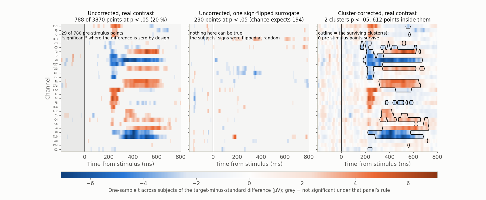
TODO(confirm): caption and numbers, once data/scripts/make_figures_p2.py has written /figures/pitfalls/pf-uncorrected-timepoint-tests.png and its sidecar — including the contrast and subjects used, the channel count and time window (and therefore the number of tests), the number of significant points in the real and null maps, the expected chance count, the cluster-forming threshold, the permutation count and the seed. The figure is generated from the same ds-erpcore subject-level difference waves that w-cluster-permutation-viz serves (CC BY 4.0; derived: epoched, baselined, re-referenced, resampled, averaged per subject). The description above states what the mechanism requires the figure to show; the sidecar’s own alt and caption are the authority once it exists.