Windowing, leakage and zero-padding
Spectral leakage, choosing a window, and what zero-padding does (interpolation) and does not do (resolution).
Prerequisites: L1.3 · Power spectral density
2 claims on this page are unverified. TODO(confirm) marks a specific statement the author has not yet checked against a
primary source. Everything else on this page has been reviewed. Treat a marked claim as
provisional and go to the cited source rather than quoting the sentence.
Objectives
- Explain spectral leakage
- Choose a window
- State what zero-padding does and does not do
Why this matters
Every spectrum you compute is the spectrum of a finite piece of signal, and cutting a piece out changes the spectrum. A pure tone becomes a peak with skirts; a strong low-frequency rhythm smears across the band above it; a 60 Hz line leaks into the gamma band. Windows control the leakage, at a price in resolution, and zero-padding, which many people use to “increase resolution”, does no such thing. Thirty minutes here prevents a class of over-interpretation that appears in published spectra with some regularity.
Concepts
Leakage: the cost of a finite segment
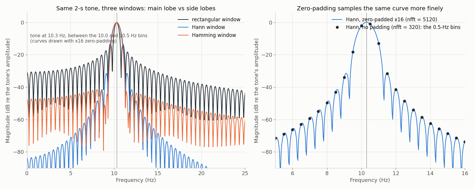
Taking N samples out of a longer signal is the same as multiplying the signal by a rectangular window that is one inside the segment and zero outside. Multiplication in time is convolution in frequency, so the spectrum you compute is the true spectrum smeared by the window’s own transform. For the rectangular window that transform is a sinc function: a main lobe two bins wide (from the first zero on one side to the first zero on the other) flanked by side lobes whose first is only about 13 dB below the peak and which decay slowly, at about 6 dB per octave (TODO(confirm) the side-lobe figures the author wants quoted; these are the standard textbook values).
Consequences you can see in the widget:
- A tone whose frequency falls exactly on a bin (an integer number of cycles in the segment) produces a single clean line, because the sinc’s zeros land on every other bin.
- A tone between bins spreads across many bins; its energy leaks. Its peak is lower, its neighbours are higher, and the side lobes extend far from it.
- A large low-frequency component (drift, delta) leaks upward into every band, raising the floor under the alpha and beta peaks; a strong 60 Hz line leaks downward into the gamma band. Leakage runs both ways.
Real EEG never has its rhythms on bins, so leakage is always present; the question is only how much and how far it spreads.
Windows: trading main-lobe width for side-lobe height
A window that tapers smoothly to zero at the segment edges removes the sharp discontinuity that the rectangular window creates, and its transform has much lower side lobes; the price is a wider main lobe. The standard choices:
| Window | Main lobe (relative to rectangular) | First side lobe | Side-lobe decay | Use |
|---|---|---|---|---|
| Rectangular | narrowest | about −13 dB | slow (about 6 dB per octave) | tone exactly on a bin; transient analysis where every sample counts |
| Hann | about twice as wide | about −31 dB | fast (about 18 dB per octave) | the default for PSD estimation (Welch) |
| Hamming | about twice as wide | about −43 dB | slow (about 6 dB per octave); side lobes stay flat far out | when the nearest side lobe matters more than the far ones (filter design, L1.5) |
| Tukey (tapered cosine) | between rectangular and Hann, set by the taper fraction | between the two | between the two | epochs with an event in the middle: tapers only the edges, leaves the centre untouched |
(TODO(confirm) the numerical side-lobe levels and decay rates in this table before promotion; they are standard values from the window-design literature, not measured on this site.)
The rule that follows: use Hann (or another smooth window) whenever you estimate a PSD, because the leakage from the aperiodic low-frequency power otherwise dominates the spectrum; use a rectangular window only when you know the content is on-bin or when you are analysing a transient and cannot afford to taper it away. Multitaper methods (L4.3) use several orthogonal tapers at once to get low leakage and low variance.
Tapering epoch edges
Tapering does more than reduce leakage in a spectrum. An epoch cut out of a continuous recording has a jump at each edge, from the data’s value to whatever comes next (zero, or the next epoch). A filter (L1.5) or a time-frequency transform (L4.2) sees that jump as a broadband event and rings around it. Tapering the edges removes the jump, at the cost of de-weighting the data near the edges; that is why Welch overlaps its segments, and why time-frequency analyses keep the events of interest away from the epoch edges.
Zero-padding: interpolation, not resolution
Appending zeros to a segment before the FFT (the nfft argument in scipy.signal.welch and numpy.fft.rfft) increases the number of bins, so the plotted spectrum has more points and looks smoother. That is all it does. The resolution of a spectrum is set by the length of the data, 1 / T (L1.2); the zeros add no information, and two tones closer together than 1 / T remain one peak however many zeros you append. What zero-padding does do is interpolate the underlying continuous spectrum of the windowed segment onto a finer grid, which is useful for one thing: reading the location of a peak more precisely than the bin spacing, because the true peak of a leaked tone may fall between bins. Used for that, with the caveat stated, it is a good tool; used to claim resolution, it is the pitfall below.
The check is simple and the widget makes it: pad a segment by a factor of four and see the curve smooth out; then add a second tone 0.3 Hz from the first with a 2-s segment and see that padding never separates them, while doubling the segment length does.
data/scripts/make_figures.py. When a spectrum looks smooth and finely resolved, look for the segment length before believing it. A 0.05 Hz grid from 2-s segments is padding; the resolution is still 0.5 Hz. A methods section that gives nfft without nperseg has not told you the resolution.
The data behind this lesson
- The widget’s real trace is the same 60-s
ds-eegbciO1 recording as L1.3 (160 Hz; ODC-By 1.0), plus a synthetic pure tone at a frequency you choose, deliberately off-bin. - The figure is generated by
data/scripts/make_figures.pyfrom a synthetic 10.3 Hz tone (no dataset); its JSON sidecar carries the parameters.
Explore

Set the tone between two bins. Compare rectangular, Hann and Hamming: watch the peak widen and the skirts fall. Raise the zero-padding and see the curve smooth without the peak narrowing. Then put a second tone 0.3 Hz away and confirm that only a longer segment separates them.
Practice
Power spectral density: periodogram versus Welch, eyes open versus eyes closed, group averaging; windows, leakage and zero-padding nb-1-3-psd
Downloads from ds-eegbci.
Section 2 of the shared L1.3 notebook computes the spectrum of an off-bin tone with each window, plots the windows and their transforms in decibels, and repeats a two-tone example with and without zero-padding and with a doubled segment length.
Exercises
Exercise ex-1-4-which-is-rectangular
Multiple choiceThe figure above shows the spectrum of the same off-bin tone computed with three windows, drawn without labels. One of them used a rectangular window. Which description picks it out?
Pitfalls
Zero-padding mistaken for resolution
- Symptom
- Smooth spectrum interpreted as finer resolution.
- Cause
Zero-padding appends zeros to a data segment before the FFT, so the transform has more bins. The extra bins interpolate the continuous spectrum of the windowed segment onto a finer grid; they add no information, because the zeros contain none. The resolution of a spectrum — the ability to separate two close frequencies — is set by the length of the data, 1 / T (L1.2): two tones closer than 1 / T…
- Detect
- Find the segment length (nperseg, or the epoch length for a single FFT) and compute 1 / T; that is the resolution, whatever the plotted grid spacing is. - Recompute the spectrum with no padding and see whether the “resolved” feature survives. - Add a synthetic second tone closer than 1 / T to a real trace and check whether the analysis pipeline reports it as separate (it should not). - Read the…
- Fix
- State resolution as 1 / T from the data length, and report nperseg (or epoch length) alongside any nfft. - Use zero-padding for what it does: reading a peak’s location more precisely than the bin spacing when the true peak lies between bins, and producing smooth plots — and say so. - When a question needs finer resolution, use longer segments (and accept the variance cost, L1.3) or longer epoch…
In other tools
In other toolsEEGLAB · FieldTrip — names only
The equivalents of what this lesson does, for a reader who works in another toolbox. Function names only: their own documentation is the place to learn how to call them.
EEGLAB
spectopo(winsize/nfft)EEGLAB
FieldTrip
ft_freqanalysis(taper/pad)FieldTrip
Names checked 2026-09-18 against EEGLAB 2026.0.0 (plugins at the versions in EEGLAB’s own plugin list) and FieldTrip 20251218.
Reading
- Cohen (2014). Analyzing Neural Time Series Data. unverified