Volume conduction: the central problem
One source produces high zero-lag coherence across all sensors; why that invalidates naive sensor connectivity, and what survives.
Prerequisites: L0.1 · What EEG measures, L4.5 · Phase, ITC and cross-frequency coupling
3 claims on this page are unverified. TODO(confirm) marks a specific statement the author has not yet checked against a
primary source. Everything else on this page has been reviewed. Treat a marked claim as
provisional and go to the cited source rather than quoting the sentence.
Objectives
- Show that one source produces high zero-lag coherence across all sensors
- Explain why this invalidates naive sensor connectivity
- List what survives volume conduction
Why this matters
Two scalp electrodes twenty-eight centimetres apart, with exactly one generator in the head and nothing else happening, have a coherence of 1. Not “high”, not “about 1” — exactly 1, at every frequency, for any recording length. Every sensor-space connectivity result you will ever read has that number sitting underneath it, and the whole of Level 5 is about what you can still say once you know it.
Concepts
Volume conduction is instantaneous, linear mixing
At EEG frequencies the head is, to an excellent approximation, a quasi-static resistive volume: capacitive and inductive effects are negligible below a few kilohertz, so the potential at every electrode is a function of the source currents at that instant, with no propagation delay. TODO(confirm): the quasi-static approximation and the frequency range over which it holds should be checked against a primary source before publication; (Nolte et al., 2004) and the Level 0 reading are the starting points.
Two consequences follow, and everything else in this lesson is a restatement of them.
It is linear. Sensor i sees a fixed weighted sum of every source: x_i(t) = Σ_k a_ik · s_k(t). The weights a_ik — the leadfield — depend on where the source is, how it is oriented, and the geometry and conductivity of the head (L5.4). They do not depend on time, on frequency, or on what the source is doing.
The weights are real numbers, not complex ones. There is no delay and no filtering in the mixing, so a_ik is a plain scalar, with a sign. A sensor on the far side of the head from the source does not see a delayed copy of the source; it sees a smaller copy, sometimes with the opposite sign.
One source makes every pair perfectly coherent, and here is why
Suppose there is exactly one source. Then x_i(t) = a_i · s(t) for every sensor, with a_i a real number. Take the Fourier transform of a segment: X_i(f) = a_i · S(f), again for every sensor, because multiplying by a constant commutes with the transform. Now form the Welch estimate of magnitude-squared coherence over K segments:
Ŝ_ij = Σ_b X_i(b) X_j*(b) = a_i a_j · Σ_b |S(b)|²
Ŝ_ii = a_i² · Σ_b |S(b)|²

γ̂²_ij = |Ŝ_ij|² / (Ŝ_ii · Ŝ_jj)
      = (a_i a_j)² (Σ|S|²)² / (a_i² a_j² (Σ|S|²)²)
      = 1
The a’s cancel. The Σ|S|² cancels. What is left is 1 — identically, not approximately.
Read what that derivation does not depend on: it does not depend on the two sensors being close together, on the source being a sinusoid, on the frequency you evaluate it at, on how many segments you average, or on the amplitudes being similar. It is not a property of this montage, this head model, or this simulation. It is arithmetic: the numerator and the denominator of the coherence estimate are the same number, because both sensors carry a real scalar multiple of one waveform. Any pair of sensors, any distance, any waveform, any K.
This is why the result belongs in the derivation and not in a table of measurements. The widget lets you watch it happen; it does not establish it.
A coherence of 1 between distant electrodes is the expected result of a single generator, not evidence of a network. The same holds for phase-locking value, amplitude correlation, and any other symmetric measure that is blind to phase lag: with one source the two sensors are the same signal, so every such measure is at its ceiling.
What the shipped montage actually shows
The widget places a homogeneous conducting sphere (radius 9 cm, conductivity 0.33 S/m) with 21 electrodes — the classic 19 of the 10-20 system plus Fpz and Oz — and its default configuration is one radial source on the occipital midline, 10 Hz, 50 nA·m, 20 s at 250 Hz, read over 2-s non-overlapping Hann segments.
Fp1 and O2 are the farthest pair that montage offers: 27.88 cm apart across the scalp, which is 18.0 cm in a straight line through the head — very nearly antipodal. Fp1 receives 5.06× less of the source than O2 does, and with the opposite sign: the scalp amplitudes are Oz 19.32 µV, O2 10.00 µV, O1 9.69 µV, Pz 5.78 µV, Cz −1.01 µV, Fp1 −1.97 µV. Every one of the 210 sensor pairs, including that one, has coherence 1.0000.
Noise dilutes the result; it never creates it
Add independent noise at each electrode — x_i = a_i·s + n_i — and the coherence in a frequency bin becomes
γ² = ρ_i · ρ_j with ρ_i = SNR_i / (1 + SNR_i)where SNR_i is the source-to-noise power ratio at that sensor in that bin, and ρ_i is therefore the share of that sensor’s power which came from the source. Equal signal-to-noise at both sensors gives γ² = (SNR/(1+SNR))²: SNR 1 gives 0.25, SNR 3 gives 0.5625, SNR 9 gives 0.81.
On the shipped defaults, sensor noise walks the Fp1–O2 pair down like this — estimate first, the formula’s prediction second:
| Sensor noise (µV SD) | Estimated coherence | Predicted ρ_i·ρ_j |
|---|---|---|
| 0 | 1.0000 | 1.0000 |
| 5 | 0.9340 | 0.9258 |
| 10 | 0.8038 | 0.7556 |
| 20 | 0.5585 | 0.4277 |
Two things to take from the table. First, the direction: independent noise lowers coherence. It is the only term in the whole simulation that is not shared between sensors, so it is the only thing working against the ceiling. A low sensor-space coherence therefore means “these two channels have poor signal-to-noise”, which is not the same statement as “these two regions are not communicating”. Second, the estimate sits consistently above the prediction, by roughly (1 − γ²)/K. That gap is finite-sample bias, not a disagreement with the formula, and it is the subject of the next section.
The independence floor: 1/K, not zero
Coherence estimated from K averaged segments is biased upward, and for two genuinely independent signals its expected value is 1/K — not zero. With ten segments, independence looks like 0.1. With four, it looks like 0.25. With a single segment the estimate is identically 1 for any two signals whatsoever, which is why the widget warns below four segments and prints the floor beside every matrix.
This matters more than it sounds. A connectivity matrix computed from short epochs has a high floor everywhere, and a paper that reports “coherence of 0.2” without reporting K has not reported anything. Any threshold for “connected” has to be referred to the floor the estimator carries, and the only honest way to know it is to compute the null for the exact estimator and the exact data length you used — which is what surrogate testing does (L5.2).
Two independent sources do not fix it
The obvious hope is that the perfect-coherence result is an artifact of having only one generator. It is not. Put two sources in the head with independent waveforms and no sensor noise at all, and each electrode sees a different mixture of both. Two mixtures of two independent signals are still correlated, because they share terms.
On the shipped montage, two independent narrowband sources with no noise give a mean coherence of 0.568 across the 210 pairs, a minimum of 0.010 — and 0.892 for Fp1 and O2, the two most distant electrodes on the head. That is the number a sensor-space connectivity paper would be reporting as a strong long-range connection. There is no connection. There are two generators that share nothing.
A trap worth knowing while you explore: two pure tones at the same frequency are perfectly coherent by construction, whatever else is true of them, so a two-tone configuration cannot demonstrate independence at all — it returns 1.0000 for every pair. Switching the source waveform to narrowband noise gives each source its own independent draw, and what is left between the sensors is mixing and nothing else.
Nor does a realistic background help. Fill the sphere with 40 independent dipoles scaled to 15 µV mean sensor RMS alongside one source, and the mean sensor coherence at 10 Hz is 0.345 against a floor of 0.100 — three and a half times the floor. Independent in the brain is not independent at the scalp.
The signature of mixing is zero lag
Everything above has one structural feature: because the weights are real, the mixed signals are in phase or in antiphase, never anything in between. The cross-spectrum of two volume-conducted copies of one source is a real number; its imaginary part is zero.
That is the opening this level walks through. A measure that discards the real part of the cross-spectrum — the imaginary part of coherency — cannot be driven by instantaneous mixing at all, because there is nothing there to drive it. In the widget, with one source, the imaginary view is zero everywhere while the magnitude-squared view is uniformly 1. Add a second source at the same frequency with a 90° phase difference and the imaginary part comes alive while the magnitude stays at its ceiling: the largest |imaginary coherency| over the montage reaches 0.9925, at F7–C4.
The price is real and L5.2 is where it is paid: discarding the zero-lag component also discards any genuine zero-lag interaction, and real neural interactions at short conduction delays sit close to zero lag. Robustness to mixing is bought with sensitivity to a class of true effects.
What a local signal looks like when it really is local
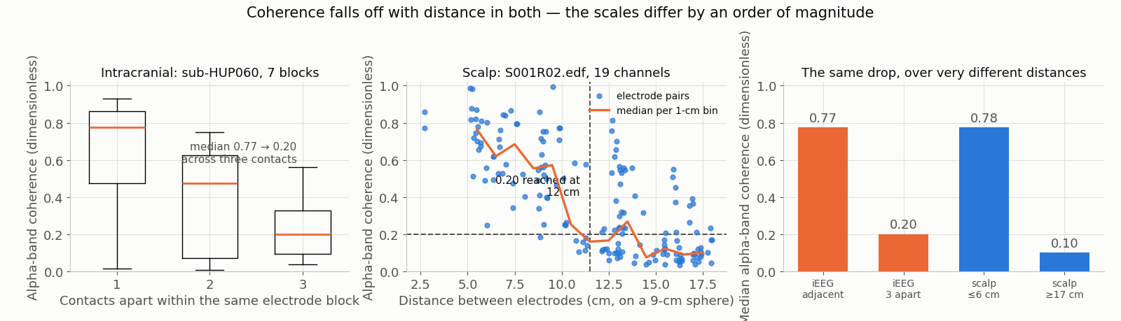
data/scripts/make_figures_p3.py. The counterpoint is the point. Scalp coherence is not flat with distance — it does fall — but the length scale over which it falls is the width of a head. Inside the skull, three contacts on one electrode shaft are already down to 0.20. Sensor-space coherence between scalp electrodes is a statement about a very coarse neighbourhood, and mostly about mixing.
Note the last caveat in the caption, because it recurs for the rest of the level: coherence is reference-dependent. The same recording gives medians of 0.78 near / 0.10 far under its own reference and 0.56 / 0.38 under an average reference of the same 19 channels. The reference is not a display choice here; it changes the numbers you would publish (pf-reference-changes-everything, L2.3).
What survives
Four routes out, in the order the level takes them:
- Measures that are insensitive to zero-lag mixing — the imaginary part of coherency, the phase-lag index and the weighted phase-lag index, and orthogonalized amplitude-envelope correlation. They cannot be produced by instantaneous mixing; they can still be reduced by it, and they cannot see genuine zero-lag coupling (L5.2).
- Spatial transforms that sharpen before you measure — the surface Laplacian and current source density, which suppress the broad spatial patterns that mixing produces and are reference-free into the bargain (L5.3).
- Source estimation, which models the mixing explicitly and inverts it — subject to its own, larger, set of assumptions (L5.4, L5.5) and to leakage, which is volume conduction reappearing in source space (L5.6).
- Designs and contrasts that difference the mixing away — comparing conditions recorded through the same head, so the leadfield is common to both. This is the cheapest of the four and the most under-used.
The data behind this lesson
- The widget is synthetic: an analytic homogeneous-sphere forward model and MNE’s
standard_1005electrode positions, re-centred and scaled, with no recording involved. It is not a model of a head; it is a model of mixing, and the sphere is what makes the arithmetic checkable. A real head has a skull, so it attenuates and blurs more than this — the mixing shown here is, if anything, an understatement (L5.4). - The widget’s forward model reproduces MNE-computed potentials for four dipoles on this montage to a worst case of 0.016 % of each row’s peak, and its two independent evaluations of the same integral agree to better than 1e-9 relative. The numbers quoted above are pinned by the widget’s own tests.
- The figure uses
ds-hup(HUP iEEG Epilepsy Dataset, CC0, OpenNeuro ds004100) andds-eegbci(EEGMMIDB, ODC-By 1.0, PhysioNet). TODO(confirm):ds-eegbci’s online reference is not documented in the site’s catalogue entry, and coherence is reference-dependent, which is why the figure reports the average-referenced medians alongside. - The dipole moments used here (20–50 nA·m) were chosen so the scalp amplitudes land in the tens of microvolts, the range a learner recognises. TODO(confirm): the moment a cortical patch of a given size actually carries is a physiological number this site has not sourced, and a skull-free sphere produces a larger scalp potential per unit moment than a real head does.
Explore

What to look for
- The matrix opens uniformly at 1.000, including Fp1–O2, the farthest pair on the head. Read the two traces above it: very different amplitudes, identical shape. Coherence does not measure amplitude.
- Raise the sensor noise and watch the fall, and check the predicted value printed beside the estimate. The prediction is built from the share of each sensor’s power that came from the source, so what is dropping is signal-to-noise, not connectivity.
- Find the independence floor in the read-out and then shorten the record or lengthen the segments until it rises. Decide for yourself what coherence value you would have called “a connection” before you saw the floor move.
- Switch the waveform to narrowband and turn on the second source. Two generators that share nothing still leave the most distant sensors at roughly 0.89. Then switch the matrix to the imaginary part and watch it collapse to nothing — that is the measure that knows the difference.
- Switch the background to independent brain sources. Sources that are independent where they are generated arrive mixed at the scalp, and the mean coherence stays several times above the floor.
Practice
Volume conduction: the widget rebuilt in Python — why one source gives coherence exactly 1 between any two sensors, what sensor noise does to that, and the intracranial counterpoint nb-5-1-vc-sim
The notebook rebuilds this simulation in Python with an explicit forward model, so that the one-source result is something you compute rather than something you are shown, and reproduces the intracranial counterpoint figure from ds-hup against neighbouring scalp channels in ds-eegbci.
Exercises
Exercise ex-5-1-single-source-coherence
NumericOne source in the head, no sensor noise. What is the magnitude-squared coherence between the two most distant sensors on the montage — Fp1 and O2, 27.88 cm apart, where Fp1 receives 5.06 times less of the source than O2? Give the value to three decimal places.
Exercise ex-5-1-independence-floor
NumericTwo genuinely independent signals, magnitude-squared coherence estimated from K = 10 averaged segments. What value do you expect?
Exercise ex-5-1-what-survives
Multiple selectWhich of these measures CANNOT be driven by instantaneous volume conduction alone — that is, which would be zero if the only thing relating two sensors were a shared source with no lag? Select all that apply.
Pitfalls
Zero-lag connectivity from one source
- Symptom
- All sensors coherent; connectivity maps mirror power maps.
- Cause
Volume conduction is instantaneous, linear mixing: every electrode sees a fixed weighted sum of every source, with real weights and no delay (L5.1). With a single generator, each sensor’s signal is xi(t) = ai · s(t) — one waveform times a real number. Take the Fourier transform of a segment and Xi = ai · S, so the coherence estimate is
- Detect
- Plot the independence floor on the same colour scale as the matrix. 1/K where K is the number of averaged segments. If the floor is visible next to the data, most of this pitfall becomes self-diagnosing. - Compare the connectivity map with the power map. If the “network” is wherever the band is strong, the null hypothesis is one generator, and it has not been tested. - Compute the imaginary par…
- Fix
- Report a measure that instantaneous mixing cannot manufacture: imaginary coherence, PLI or wPLI for phase, orthogonalized amplitude-envelope correlation for envelopes. State in the same sentence that these are blind to genuine zero-lag coupling, so that a null result is reported as uninformative about instantaneous interaction rather than as absence of connection. - Sharpen before measuring. Th…
In other tools
In other toolsFieldTrip — names only
The equivalents of what this lesson does, for a reader who works in another toolbox. Function names only: their own documentation is the place to learn how to call them.
FieldTrip
ft_dipolesimulationFieldTripft_connectivitysimulationFieldTrip
Names checked 2026-09-18 against FieldTrip 20251218.
Reading
- Bastos & Schoffelen (2016). Connectivity tutorial review. unverified
- Nolte et al. (2004). Imaginary coherence. unverified