Zero-lag connectivity from one source

Symptom

A sensor-space connectivity matrix is almost uniformly high: nearly every electrode pair is “connected”, including pairs on opposite sides of the head, and the values sit far above whatever threshold was chosen. The connectivity map looks like the power map — wherever the band is strong, the connections are strong — and the strongest “network” sits under the strongest generator. The pattern barely changes between conditions, between subjects, or between rest and task. A “long-range network” is reported between frontal and posterior sites in the same band as the dominant rhythm. In source space the same thing recurs one level up: the parcels with the most estimated power are the parcels with the most connections.

Cause

Volume conduction is instantaneous, linear mixing: every electrode sees a fixed weighted sum of every source, with real weights and no delay (L5.1). With a single generator, each sensor’s signal is x_i(t) = a_i · s(t) — one waveform times a real number. Take the Fourier transform of a segment and X_i = a_i · S, so the coherence estimate is

γ̂²_ij = |a_i a_j Σ|S|²|² / (a_i² Σ|S|² · a_j² Σ|S|²) = 1

The scale factors cancel. The result is exactly 1, for every pair, at every frequency, over any number of averaged segments, at any distance, for any source waveform. It is not an approximation and not a property of a particular montage: it is what the coherence estimator computes when both inputs are scalar multiples of one signal.

Four corollaries account for everything in the symptom list:

Amplitude does not matter, so distance does not save you. On the site’s 21-site simulation the two furthest electrodes — Fp1 and O2, 27.88 cm apart across the scalp, 18.0 cm in a straight line — still give 1.0000 with no noise, even though Fp1 receives 5.06 times less of the source than O2 does.
Two independent sources do not fix it. Each electrode sees a mixture of both, and two mixtures of two independent signals are still correlated. Two independent narrowband sources with no noise give a mean coherence of 0.568 across the 210 pairs on that montage, and 0.892 for the most distant pair.
A realistic background does not fix it. Forty independent dipoles inside the head, scaled to 15 µV mean sensor RMS alongside one source, leave the mean sensor coherence at 0.345 against an independence floor of 0.100. Independent in the brain is not independent at the scalp.
The floor is not zero. Coherence estimated from K averaged segments has an expected value of 1/K for genuinely independent signals — 0.1 at ten segments, 0.25 at four, and identically 1 at one. A matrix “thresholded at 0.2” with five segments has thresholded at the floor.

Three further mechanisms produce the identical signature and are commonly mistaken for it, or for each other:

A reference carrying signal. Every channel is electrode minus reference, so a reference that is not electrically silent injects one shared term into every pair at once (pf-reference-changes-everything).
Rank deficiency after cleaning. Removing ICA components and back-projecting, or interpolating a bad channel, makes some channels arithmetic combinations of others (pf-interpolation-rank). An interpolated channel’s coherence with its neighbours is partly an identity.
Source leakage. Source estimation applies a fixed linear operator to the sensors, so two source estimates share sensor data by construction (L5.6). The mixing is redistributed and relabelled with anatomical names, not removed — which makes the same artifact more persuasive.

Detect

Plot the independence floor on the same colour scale as the matrix. 1/K where K is the number of averaged segments. If the floor is visible next to the data, most of this pitfall becomes self-diagnosing.
Compare the connectivity map with the power map. If the “network” is wherever the band is strong, the null hypothesis is one generator, and it has not been tested.
Compute the imaginary part of coherency, or wPLI, on the same data. Instantaneous mixing has no lag, so it cannot produce either. A connection that vanishes entirely under a lag-based measure is consistent with pure mixing (L5.2) — remembering that the converse is not a clean result, since a genuine zero-lag interaction also vanishes.
Re-run under a second reference. Coherence is reference-dependent, and a pattern that reorganises when the reference changes was partly the reference. On one 19-channel eyes-closed recording the median near-pair and far-pair alpha coherence goes from 0.78 / 0.10 under the delivered reference to 0.56 / 0.38 under an average reference of the same channels.
Check the rank of the data after cleaning against the channel count, and list which channels were interpolated. Exclude interpolated channels from the matrix.
Build a surrogate null through the whole pipeline — filtering, epoching, normalisation, and the inverse and parcellation if there is one — rather than comparing against zero.
Look at the coherence-versus-distance curve. Real scalp coherence falls with distance, over about the width of a head. A curve that is flat is mixing plus a reference; a curve that falls over millimetres is not scalp EEG.

Fix

Report a measure that instantaneous mixing cannot manufacture: imaginary coherence, PLI or wPLI for phase, orthogonalized amplitude-envelope correlation for envelopes. State in the same sentence that these are blind to genuine zero-lag coupling, so that a null result is reported as uninformative about instantaneous interaction rather than as absence of connection.
Sharpen before measuring. The surface Laplacian is reference-free and suppresses the broad spatial patterns mixing produces (L5.3). It composes with wPLI; neither replaces the other.
Handle the reference explicitly — report it, and report the sensitivity of the result to it.
Exclude interpolated channels and report the rank of the cleaned data.
In source space, quantify leakage rather than assuming it away. The cross-talk between the specific pair you are claiming is computable from the inverse operator and the leadfield with no data at all; compute it, report it, and apply orthogonalization while stating what it removed along with the artifact (L5.6).
Prefer within-study contrasts. A difference between two conditions recorded through the same head shares its mixing, so much of the artifact cancels — which is far more than a raw connectome can claim.
Correct for the number of pairs. 21 channels give 210, 64 give 2016, 68 parcels give 2278.
Write the claim at the strength the measure supports. “wPLI in 8–12 Hz differed between conditions over these channels” is a result; “frontoparietal connectivity” is an interpretation that needs the alternatives ruled out first.

Example

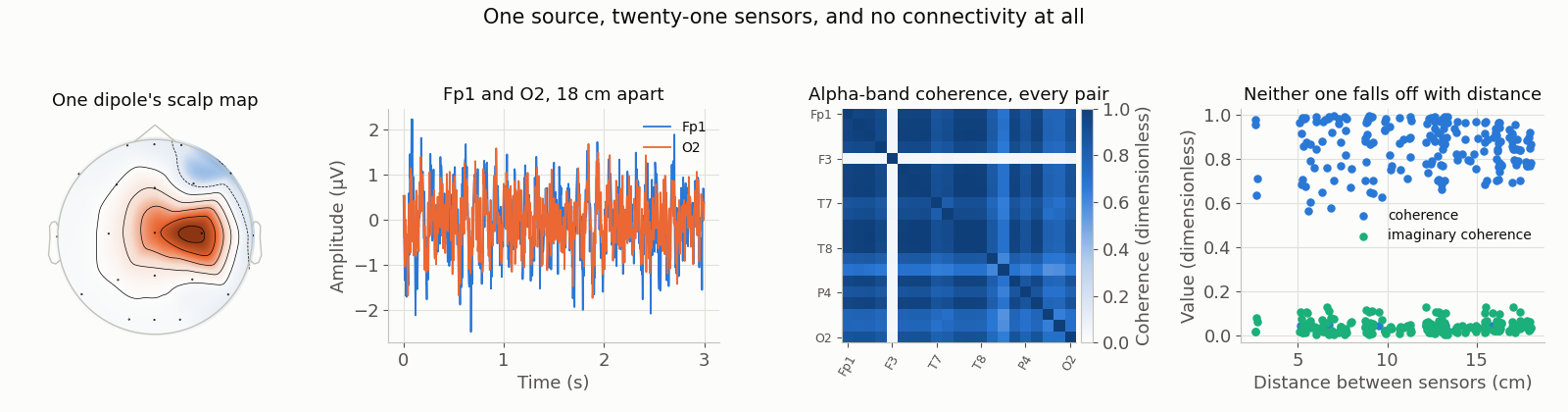
Simulated, not recorded: one 10 Hz dipole in a homogeneous conducting sphere (radius 9 cm, conductivity 0.33 S/m), 21 electrodes, independent white sensor noise of 0.5 µV. Median alpha-band coherence over all 210 sensor pairs is 0.87; the two most distant electrodes (Fp1 and O2, 18 cm apart in a straight line through the head, 27.88 cm across the scalp) reach 0.87. There is exactly one generator, so every one of those numbers is mixing. Median imaginary coherence is 0.036, because instantaneous mixing has no lag — which is why the lagged measures are the ones worth reporting. The one pale row and column in the matrix is F3, which happens to sit on the map’s zero line: the source projects onto it hardly at all, so its trace is mostly sensor noise and its coherence with everything else collapses (minimum 0.04). That is the only structure in the whole matrix, and it is electrode geometry, not a network. Welch estimate, 1024-sample Hann segments at 250 Hz with 50 % overlap, 60 s, seed 20260918. Generated by data/scripts/make_figures_p3.py.

Two details of the figure are worth reading twice. The coherence here is 0.87 rather than 1.00 only because 0.5 µV of independent sensor noise was added; with no noise every cell of that matrix is exactly 1.000, which is the result w-volume-conduction-sim opens on. And the single “interesting” feature — the one pale channel — is the most instructive thing in the picture: it is the channel the source happens not to project onto, and in a real dataset it would be the one a reader’s eye went to.