Time-frequency edge artifacts in the baseline

Symptom

The bottom rows of a time-frequency map ramp up toward one or both ends of the epoch, in a smooth arc that is widest at the lowest frequency. The pre-stimulus interval looks unusually powerful. After baseline normalization the whole map sits below zero — an event-related desynchronization at every frequency and every latency, including where nothing happened — or the effect of interest is oddly weak. The same analysis on a longer epoch, cropped afterwards to the same window, gives a different answer. Cutting the epoch shorter makes the ramp worse; padding it out makes the ramp disappear from view without changing the numbers in the reported window.

Cause

A time-frequency estimate at time t is a weighted sum of the signal over the estimator’s whole support around t. Near either end of the epoch part of that support falls outside the data, and the transform reads whatever the implementation puts there — zeros, a mirrored copy, the epoch’s own mean. The result is not random noise; it is a systematic distortion with a characteristic shape.

Its width is set by the estimator, and it is widest exactly where it does the most damage:

For a Morlet wavelet, σ_t = n_cycles / (2π f). Two conventions for the affected half-width are in use and both must be named when quoted: MNE truncates its kernel at 5 σ_t, and a 2 σ_t cone of influence is the more permissive alternative. Either way the region grows in proportion to the cycle count and inversely with frequency.
For multitaper, it is half the analysis window, n_cycles / (2 f).
For filter-Hilbert, it is the reach of the filter: (numtaps − 1) / sfreq for a zero-phase FIR run in both directions.

Two facts make this a pitfall rather than a nuisance. First, the region is far larger than people expect at low frequencies: at 4 Hz with 7 cycles it is 0.56 s per side under the 2 σ convention and 1.39 s under the 5 σ one, and at 3 Hz with 7 cycles the 5 σ region is 1.86 s per side — so a 3-second epoch has no sample at 3 Hz that is free of padding. Second, the baseline window usually sits at the very start of the epoch, which is the contaminated region. Normalization divides the entire map by that baseline, so a locally inflated divisor becomes a global bias: every cell, at every frequency and latency, is scaled by a number the recording did not produce.

Padding does not fix it. Zero-padding moves the boundary between “reading data” and “reading zeros” out of the plotted range without creating the data the estimator needs. Reflection padding is worse in one respect: it invents a mirror-symmetric continuation, which at an epoch boundary has a specific, artificial phase relationship to the real signal.

Detect

Compute the margin before you plot anything. From the cycle scheme and the lowest analysed frequency, work out the affected half-width, state which convention you used, and compare it with the distance from the epoch edge to the baseline window and to the reporting window. If the margin reaches either, you have the problem.
Transform the same window twice, from two epoch lengths. Cut a wide epoch and a narrow one around the same event, transform each at its own length, crop both to the same reporting window and subtract. Inside the margin the difference is large; outside it, it is nothing. On the figure below the median absolute difference at 4 Hz is 84 % inside the cone of influence and 0.0 % outside it.
Look at the un-normalized map. The ramp is obvious in raw power and invisible after a baseline has folded it into every cell.
Plot the margin on the map. Shade it per frequency row rather than as one vertical band; it is a curve, not a rectangle, and drawing it as a rectangle hides that the low rows are worse.
Watch what the baseline does to a null region. If a frequency and latency where nothing is expected shows a consistent offset after normalization, the divisor is suspect.

Fix

Cut the epoch wider than the window you intend to report, transform at that length, and crop afterwards. The reporting window needs a clear margin at each end, computed from the widest wavelet in the analysis. This is the fix; the rest are mitigations.
Place the baseline entirely outside the margin, and end it early enough that the estimator’s forward smoothing has not already pulled post-event data into it.
Where the data cannot be widened, in order of preference: ramp the cycle count down at low frequencies so the wavelet is shorter where it is longest; raise the lowest analysed frequency until the margin fits, and say what band was therefore not analysed; or drop the affected rows from the figure and from the statistics rather than plotting values you know are padding.
Exclude the margin from the tested space in any statistic. Testing inside it tests the padding, and a cluster that lives in the margin is an artefact of the transform (L4.7).
Report all of it: the epoch length actually transformed, the reporting window, the cycle scheme as a formula, the margin as a number, the convention behind that number, and the baseline window with its distance from the margin.

Example

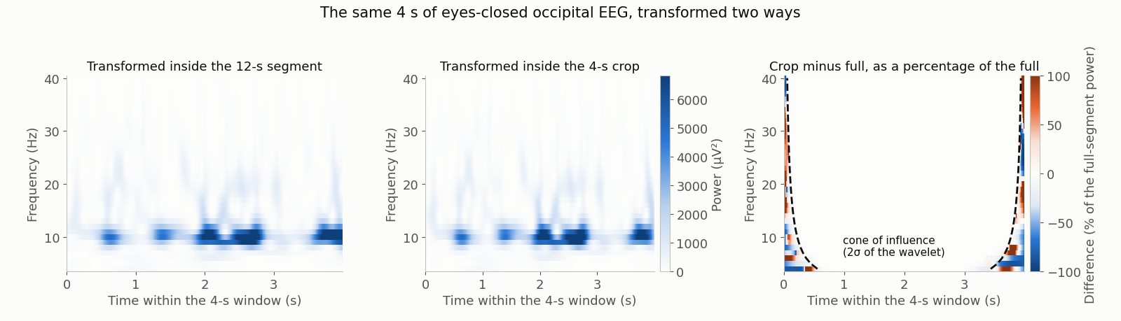
Edge effects are not noise; they are the transform running out of data. The same 4 seconds of ds-eegbci S001R02 (O1, eyes closed, 160 Hz) gives different power at 4 Hz depending only on whether the samples on either side were available: a median absolute difference of 84 % inside the cone of influence against 0.0 % outside it. The dashed lines are two standard deviations of the wavelet’s Gaussian envelope, 2·n_cycles/(2πf) with 7 cycles — 0.56 s at 4 Hz, 0.22 s at 10 Hz, 0.11 s at 20 Hz, 0.06 s at 40 Hz — so at 4 Hz a 1-second epoch has no usable estimate anywhere in it. The difference panel’s colour scale is clipped at ±100 %: at the very first and last samples the difference is far larger, but there the full-segment power is near zero and the percentage says more about division than about the transform. Computed with mne.time_frequency.tfr_array_morlet (7 cycles, zero_mean=True, use_fft=True); generated by data/scripts/make_figures_p3.py. ds-eegbci is ODC-By 1.0, open access, DOI 10.13026/C28G6P; this is a derivative — cropped, average-referenced and transformed.

Crop wide, transform, then crop to the window you meant.