STFT and Morlet wavelets

Why this matters

A time-frequency map is not a measurement of the data; it is the data seen through a window you chose, and the two numbers that define that window — frequency and cycles — set how much time and how much frequency get blurred together in every cell. Choose them without knowing what they do and the map will still look convincing. Worse, the same two numbers decide how far into each end of your epoch the estimate is made of padding rather than of signal, and that region is usually where the baseline sits.

Concepts

The short-time Fourier transform

The Fourier transform of a whole epoch says which frequencies are present and says nothing about when. The obvious repair is to cut the epoch into short windows, transform each one, and slide along: the short-time Fourier transform. Everything about time-frequency analysis follows from what that repair costs.

A window of length T seconds has a frequency resolution of 1/T Hz — the same relation L1.3 and L1.4 established for Welch’s method, because the STFT is Welch’s method with the averaging turned off and the segment index kept as a time axis. A 0.5 s window resolves 2 Hz; to resolve 0.5 Hz you need 2 s of data in every estimate, and every estimate is then a statement about 2 s of time. You cannot buy both: the product of the temporal and spectral widths of any window has a positive lower bound, reached by the Gaussian.

The STFT’s characteristic property is that the window is the same length at every frequency. That is efficient and it is rarely what a neural question wants. At 4 Hz, a 0.25 s window is one cycle — too short for the frequency to mean much. At 60 Hz, the same window is fifteen cycles — far longer than any burst you would hope to localise. So the standard choice in this field is a window whose length is specified in cycles, which is what the Morlet wavelet gives.

The Morlet wavelet

A complex Morlet wavelet at frequency f is a complex sinusoid multiplied by a Gaussian envelope:

w(t) = C · exp(2πi f t) · exp( −t² / (2 σ_t²) ),     σ_t = n_cycles / (2π f)

Convolving the signal with it gives a complex-valued time course per frequency: magnitude squared is power, the angle is phase (L4.5). The single parameter n_cycles fixes the envelope width in units of the period, so a wavelet at 40 Hz with 7 cycles is a quarter the duration of a 10 Hz wavelet with 7 cycles.

Two widths follow, and both are quoted as full width at half maximum rather than as σ:

FWHM_t = 2 σ_t √(2 ln 2)  =  n_cycles · √(2 ln 2) / (π f)
σ_f    = 1 / (2π σ_t)     =  f / n_cycles
FWHM_f = 2 σ_f √(2 ln 2)  =  2 f √(2 ln 2) / n_cycles

Which FWHM you mean has to be said out loud. The relations above are the widths of the Gaussian amplitude envelope, which is what mne.time_frequency.fwhm returns and what the widget quotes by default. The width of the power envelope — the squared Gaussian — is a factor √2 narrower. At 10 Hz with 7 cycles the amplitude convention gives 262.3 ms and 3.364 Hz; the power convention gives 185.5 ms and 2.379 Hz. Neither is wrong; a number without its convention is ambiguous by 41 %.

Under the amplitude convention the product is a constant for every frequency and every cycle count:

FWHM_t · FWHM_f = 4 ln 2 / π = 0.8825 s·Hz

That constant is the trade-off. Cycles do not buy resolution; they spend it on one axis to gain it on the other. Raising the cycle count makes the wavelet longer in time and narrower in frequency, in exact proportion.

Choosing cycles by frequency

Three schemes are in common use, and the choice is a statement about what you are looking for rather than a correctness question:

• A fixed cycle count at every frequency. Simple to state and to reproduce. Because σ_t ∝ 1/f, the temporal resolution automatically sharpens with frequency, which usually matches what you want — but at the bottom of the map a fixed count can be unusable: a 7-cycle wavelet at 3 Hz has seven periods spanning 2.33 s, a half-amplitude width of 0.874 s, and a support of 3.71 s at the ±5 σ truncation below.
• A cycle count that ramps with frequency — for example from 3 cycles at the bottom of the axis to 10 at the top. Keeps low-frequency estimates temporally usable at the cost of frequency detail there, and buys frequency detail up high where there are cycles to spare.
• A fixed window length in seconds — which is the STFT again, expressed as n_cycles = f · T.

The shipped epoch’s own scheme, recorded in its sidecar, is n_cycles = max(3, f/2): three cycles up to 6 Hz, then a ramp. Whichever you use, it goes in the methods section as a formula, not as a word, because the smoothing it implies at each frequency is what the reader needs in order to know what the map’s cells mean.

Edge effects, and why they land in the baseline

A convolution at time t reads the signal over the wavelet’s whole support around t. Near either end of the epoch some of that support falls outside the data, and the transform reads whatever is there — zeros, mirrored samples, whatever the padding does. The result is not noise; it is a systematic distortion, usually a ramp, and it is worst at low frequencies because that is where the wavelet is longest.

How wide the affected region is depends on the convention for “the wavelet’s support”, and again the convention has to be stated:

• MNE truncates the kernel at ±5 σ_t, where the envelope is 3.7 × 10⁻⁶ of its peak, and the widget shades that half-width at each end. For the shipped epoch’s scheme this is 0.597 s per side, set by the 4 Hz row.
• A ±2 σ_t cone of influence is the more permissive convention, and is the one drawn in the pitfall figure below: 0.557 s at 4 Hz with 7 cycles, 0.223 s at 10 Hz, 0.111 s at 20 Hz.

Either way the number grows with cycles and falls with frequency, and either way a 3-second epoch analysed at 3 Hz with 7 cycles has no sample free of padding: 5 σ_t is 1.857 s per side.

The practical consequence is the one pf-tf-edge-effects is named for. The baseline window usually sits at the very start of the epoch — which is exactly the contaminated region — so an inflated baseline divides the entire map and produces an apparent desynchronisation everywhere, including at times and frequencies where nothing happened (L4.4).

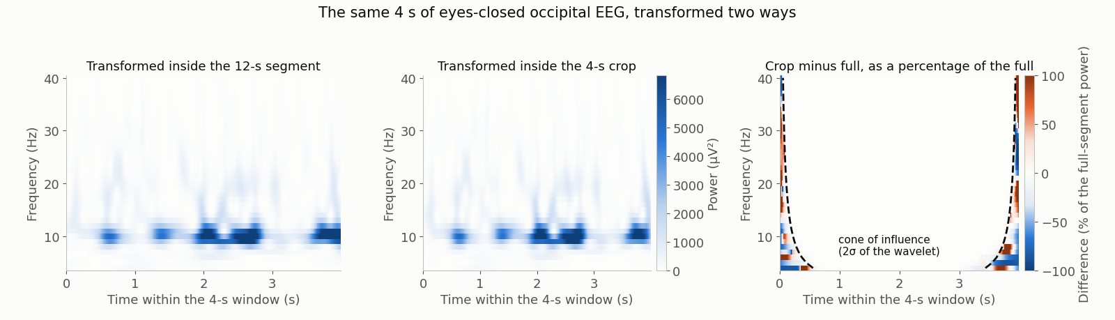
Padding is not a fix. Zero-padding an epoch to a greater length does not create the data the wavelet needs; it only moves the boundary between “reading data” and “reading zeros” out of sight. Reflection padding is not a fix either — it invents a mirror-symmetric continuation, which at an epoch boundary is a signal with a specific, artificial phase relationship to the real one. The only real fix is to cut the epoch wider than the window you intend to report, transform, and then crop to the reporting window. If the recording does not allow that — if the events are too close together, or the run ends — say so, and exclude the affected rows rather than plotting them.

The data behind this lesson

• ds-eegbci, ODC-By 1.0, open access; 64 channels, 160 Hz, no hardware filters, 60 Hz mains. The widget serves one 3-second epoch: subject S001, run R08, channel C3, a right-fist motor-imagery trial (annotation code T2), stored from −1.0 to +2.0 s around the cue, so the cue sits 1.0 s into the epoch. Average-referenced over the 64 EEG channels offline, unfiltered and unresampled at the dataset’s native 160 Hz, channel mean removed over the window.
• The trial was selected, algorithmically and on purpose. Among this subject’s T2 trials whose largest absolute sample stays below 100 µV, the one with the largest mu-band drop from −1…0 s to 0.5…2 s was taken: a 7.08 dB drop. The full ranking is in the sidecar. It is a teaching example chosen for legibility, not a sample of anything, and nothing about the cohort or about motor imagery in general follows from it.
• The Morlet map is not shipped. The sidecar’s client_morlet block records the frequency grid (4–40 Hz in 1 Hz steps), the per-frequency cycle list, zero_mean, and MNE 1.10.2’s wavelet normalisation written out in full, so the browser computes the map itself and the cycles slider is live. TODO(confirm): ds-eegbci’s own online reference is not documented in the catalogue, so the average reference is this site’s choice and is recorded as such in the sidecar.
• The notebook runs tfr_morlet on the same kind of epochs under several cycle schemes and prints the widths each one implies.

Explore

The sequence that makes the argument: set the cycles control to a fixed number and leave it at 7 with the frequency at 10 Hz — the configuration the exercise names — and read the two width figures and their product. Now drag the cycle count and watch the two widths move in opposite directions while the product stays pinned at 0.8825 s·Hz. Switch the “widths quoted as” control between amplitude and power and watch both numbers change by 41 % while the picture does not. Drop to 3 cycles and watch the mu desynchronisation sharpen in time and smear across the beta range. Finally shorten the epoch and watch the shaded margin swallow it.

Practice

The notebook computes tfr_morlet on ds-eegbci motor-imagery epochs under a fixed-cycle scheme, a ramped scheme and a fixed-window scheme, and prints the temporal and spectral FWHM each one gives at every frequency, with the convention named.

Exercises

Set the widget’s cycles control to a fixed number, leave it at 7, and set the analysis frequency to 10 Hz. Leave “widths quoted as” on its default, amplitude.