Overclaiming source depth or precision

Symptom

A results section names a deep structure — hippocampus, amygdala, thalamus, insula, anterior cingulate, brainstem — as the generator of a scalp EEG effect, on the strength of a source-estimation figure. Or the claim is superficial but the precision is not: a maximum is attributed to a specific gyrus, or two conditions are said to differ in generator location by a few millimetres, or the number of generators is read off the number of blobs in the map. Adjacent variants: an anatomical label is quoted from a source analysis while the methods do not state the head model, the regularization or the resolution; a coloured cortical surface is captioned as though it were a measurement; and cortex outside the coloured region is described as inactive.

Cause

Two facts, and they compound.

The scalp map of a deep source is reproducible by a superficial patch. Depth broadens and weakens a scalp projection; spatial extent also broadens it. The two trade off against each other, and a sparse montage cannot see the difference. In the simulation below, a single dipole 36 mm below the scalp and 61 dipoles spread over a 30-degree cap 14 mm below it produce maps correlating at r = 0.992, with a largest point-by-point difference after rescaling of 5.6 % of the peak. That is not special to one depth: for every single-dipole depth from 27 to 72 mm, a superficial patch exists whose map matches it at r ≥ 0.960. Depth does change amplitude — 10.30 µV at 27 mm against 2.16 µV at 72 mm — but source strength and source extent change amplitude too, so amplitude separates nothing on its own.

The inverse problem has a large null space. There are thousands of candidate source locations and tens of electrodes, so whole families of source configurations produce identically zero at the sensors (L5.5). Adding any of them to a solution changes nothing measurable. Two consequences follow that are routinely mistaken for evidence:

Goodness of fit proves nothing about location. A solution can explain 99 % of the sensor variance and be in the wrong place, because a wrong-place solution plus a null-space component fits exactly as well.
The estimate is the data plus a preference. Which solution you see out of the infinite set is decided by the criterion — minimum norm, depth weighting, a beamformer, a two-dipole fit — and by the regularization. Depth weighting is what makes deep solutions appear; it is a prior, not a measurement that found them.

On top of those, four amplifiers:

Point spread. Every linear estimate is smoothed: a point source produces a broad estimated blob whose width varies by an order of magnitude across the source space and is worst for deep locations. A blob is not a localization and the number of blobs is not a count of sources.
Head-model error. A template anatomy is nobody’s head, and the brain-to-skull conductivity ratio is a modelling assumption whose true value is contested. Both produce systematic, not random, localization error that does not average away across subjects.
Coregistration error translates directly into localization error and is the component most often left unreported.
Channel count and coverage. At 19 to 21 electrodes a shallow, focal, tangential source’s field is reproduced at r ≈ 0.71 with its peak amplitude understated fourfold — before any head model is chosen. A montage that stops above the ears never samples the inferior surfaces at all, and no inverse recovers a field that was not measured.

Detect

Ask what else would have produced the same scalp data. For a deep claim, the answer is always “a superficial patch”, and the figure below is the demonstration. If the analysis cannot exclude it, the claim is not supported.
Compute the point-spread function at the claimed location. It needs no data — only the inverse operator and the leadfield, Res = W·L — so there is never an excuse for not knowing it. If the point-spread width is larger than the distinction being drawn, the distinction is not in the data.
Re-run with a different inverse method and a different regularization. A claim that does not survive a change of method was a property of the method. Two methods disagreeing on the same data is the null space made visible.
Check whether depth weighting is on, and what the result looks like without it.
Read the methods for the head model, the coregistration residual, the electrode positions (template or digitized), the noise covariance and the regularization. A source figure missing any of these cannot be evaluated.
Count the channels and look at the coverage, and compare them with the spatial scale of the claim.
Watch for absence claims. “Activity was confined to region X” requires the estimate outside X to be something other than the point-spread function of the estimate inside it.

Fix

State the claim at the scale the resolution supports — lobar or broad regional, for a superficial cortical generator — and give the point-spread width at that location alongside it.
Prefer relative claims within one study. A difference between conditions computed through one pipeline shares its head-model, montage and prior errors between the two conditions, so much of the systematic error cancels. This is the strongest thing EEG source analysis does.
Do not claim a deep generator from scalp EEG alone. If the hypothesis is about a deep structure, it needs a constraint from somewhere else: simultaneous intracranial recording, a lesion or stimulation result, an fMRI-informed prior stated as a prior, or a paradigm whose scalp signature is diagnostic for independent reasons. Say which.
Report the sensitivity analysis — the result under a second method and a second regularization — rather than the single prettiest map.
Show the electrode positions on the figure and state the reference, the montage and the channel count in the caption.
Use dipole fitting where the low-dimensional assumption is independently motivated, with the goodness of fit and the confidence volume reported; and do not use a beamformer where the sources are likely to be correlated, because correlated sources cancel (L5.5).
Write the negative section. A short paragraph listing the claims a reader might draw from the figure that the analysis does not support is worth more to a careful reader than another figure.

Example

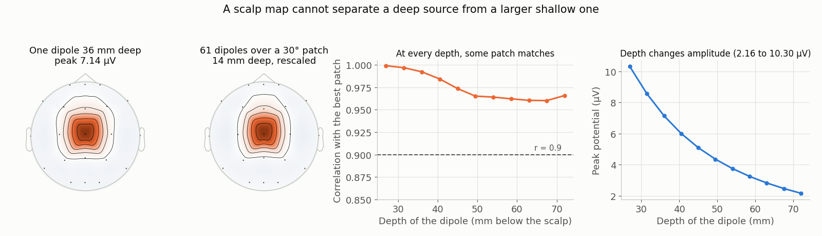
Simulated, not recorded: radial dipoles in a homogeneous conducting sphere (radius 9 cm), the 21 10-20 electrodes, average-referenced, no noise. One dipole 36 mm below the scalp and 61 dipoles spread over a 30° cap 14 mm below it give maps correlating r = 0.992; after rescaling, the largest point-by-point difference is 5.6 % of the peak. That is not special to this depth: for every single-dipole depth from 27 to 72 mm a patch exists whose map correlates at least 0.960. Depth and spatial extent trade off against each other and 21 electrodes cannot see the difference. Depth does change amplitude — 2.16 µV at 72 mm against 10.30 µV at 27 mm — but source strength and extent change amplitude too, so it separates nothing on its own. A claim that a scalp effect arose in a deep structure is a claim the sensors cannot support; it needs a constraint from somewhere else. Generated by data/scripts/make_figures_p3.py; the figure is produced only if the featured depth matches at r ≥ 0.98 and every tested depth at r ≥ 0.9, and skipped otherwise.

Two things the figure is careful about, and one it cannot do. Correlation is the right statistic here precisely because it is scale-free: the two maps differ in amplitude, and amplitude is exactly what a source’s strength and extent also control, so a comparison that included amplitude would be answering a different question. The comparison is also made with no noise at all, which is the most favourable case for telling the two apart — with realistic noise they are less distinguishable, not more. And what the figure cannot do is prove that a deep generator was absent; it shows that the measurements do not distinguish the two hypotheses, which is a statement about what can be claimed, not about what is true.