The inverse problem and source estimation

Objectives

• Explain ill-posedness
• Compute minimum-norm, dSPM and sLORETA/eLORETA estimates
• Compute an LCMV beamformer
• Describe point-spread and resolution
• State which claims EEG source estimates can defend

Why this matters

Source estimation is the most persuasive thing you can do with EEG and the easiest to overclaim with. A cortical surface in colour looks like a measurement of where the activity was. It is the output of an optimisation problem with no unique solution, and the picture you are looking at is as much a property of the criterion you chose as of the data. This lesson is about holding both facts at once: the methods are genuinely useful, and the set of claims they support is much smaller than the pictures suggest.

Concepts

Why there is no unique answer

The forward problem is a matrix: x = L·j + noise (L5.4). The inverse problem is to recover j from x. It is ill-posed in the strongest sense, for a reason that is not about noise or numerical conditioning:

There are far more unknowns than equations. A typical source space has thousands of candidate locations; a typical EEG montage has tens of electrodes. L therefore has a large null space: whole families of source configurations j₀ for which L·j₀ = 0 exactly. Add any of them to any solution and the predicted measurements do not change at all. No amount of data quality removes this — it is the rank of a matrix, not an estimation difficulty.

Those silent configurations are not mathematical curiosities. A closed-field cell arrangement produces no far field (L0.1). Two nearby dipoles in opposition largely cancel. Sources deep in the head with the right geometry produce almost nothing at the scalp. “Nothing appeared at the sensors” and “nothing happened” are different statements, and no inverse method can distinguish them.

Two practical consequences follow immediately, and both are routinely violated in print:

• Every inverse solution is the data plus a preference. The solution you get is the one your criterion selects out of an infinite set that all fit the data equally well. Change the criterion — minimum norm, minimum norm with depth weighting, a beamformer, a two-dipole fit — and you get different answers from the same data, all of them “consistent with the measurements”.
• Goodness of fit proves nothing about localization. A solution can explain 99 % of the variance in the sensor data and be in the wrong place, because a solution in the wrong place plus a null-space component explains exactly as much.

The general form: every method is a matrix

For all the linear methods in this lesson, the estimate is

ĵ(t) = W · x(t)

with W an n_sources × n_channels matrix computed once. The methods differ only in how W is chosen. That is worth internalising, because it means every linear inverse is a fixed spatial filter bank applied to the sensors — with all the consequences L5.1 attached to spatial filters, including the fact that each estimated source time course is a weighted sum of all the channels, and therefore of all the sources.

Minimum norm and its family

Minimum-norm estimation (MNE) picks the solution with the smallest total source power that fits the data to within the noise:

W = R Lᵀ (L R Lᵀ + λ² C)⁻¹

with C the noise covariance, R a source covariance (the prior), and λ² a regularization parameter. Three ingredients, three ways to be wrong:

• The noise covariance C is estimated, usually from a pre-stimulus baseline or from empty-room data. It is used to whiten the problem, so that channels with more noise count for less. A badly estimated C — too few samples for the number of channels, or a baseline that contains the effect — degrades everything downstream, and this is the single most common silent failure in practice. Regularized covariance estimators exist and should be used.
• λ² is an SNR assumption, conventionally set from an assumed amplitude SNR (λ² = 1/SNR²; SNR 3 gives λ² = 1/9). Larger λ² gives smoother, more biased, more stable maps. It is a knob, and its value belongs in the methods section.
• R is the prior, and with R proportional to the identity the method has a well-known depth bias: deep sources need larger amplitudes to produce the same scalp field, so the minimum-norm criterion prefers to explain the data with superficial sources. Depth weighting compensates by scaling the prior with the leadfield norm, which is another parameter with another choice in it.

dSPM divides each source’s estimate by the standard deviation the noise alone would produce there. The result is a noise-normalised statistic rather than a current estimate, with roughly uniform noise sensitivity across the source space, which is why dSPM maps look far less depth-biased than raw MNE maps. It is still the MNE spatial filter underneath: the smoothing is unchanged, only the scaling.

sLORETA standardizes instead by the variance of the estimate itself, which is the diagonal of the resolution matrix (below). TODO(confirm): sLORETA is frequently described as having zero localization error for a single point source in the noiseless case; that property, its exact conditions and whether it survives realistic noise and multiple simultaneous sources must be checked against a primary source before this lesson is published. eLORETA is a related weighting with a similar motivation. Neither removes the underlying smoothing: a zero-error maximum is not a sharp estimate.

Beamformers

An LCMV beamformer takes a different route. For each candidate location it designs a spatial filter that passes that location with unit gain while minimising the total output power — that is, while suppressing everything else as hard as the data allow. It is adaptive: the filter depends on the data covariance, not only on the forward model.

That buys real advantages (good suppression of interfering sources, no global smoothness prior) and one specific, severe failure mode: correlated sources cancel. If two regions are perfectly or near-perfectly correlated, the beamformer can minimise output power by subtracting one from the other, and both disappear. Bilateral homologous activation and strongly phase-locked evoked responses are exactly this case, which makes beamformers a poor default for ERP source analysis and a reasonable one for induced oscillatory activity. Like every covariance-based method, it also needs enough data to estimate the covariance, and regularization when it does not have it.

Dipole fitting is the low-dimensional alternative: assume one or two focal sources and fit their positions, orientations and amplitudes. When the assumption is defensible — an early sensory component, an epileptic spike — it is the most interpretable method available, with an explicit goodness of fit and confidence volume. When it is not, it will still return a dipole, placed wherever best compromises between several real sources.

Resolution: point spread and cross-talk

The honest way to describe what any linear method does is the resolution matrix:

Res = W · L

If the inverse were perfect, Res would be the identity. It never is.

• A column of Res is a point-spread function: put a unit source at location k and this is the whole map the method returns. Its width is the method’s spatial resolution at k; the distance from k to its maximum is the method’s localization bias there.
• A row of Res is a cross-talk function: this is where the estimate at location k actually draws its signal from. It is the same object read the other way, and it is the direct statement of leakage — the subject of L5.6.

Two things to take from this. First, resolution is not uniform: it varies by an order of magnitude across the source space, is worst for deep sources, and depends on the montage, the head model, the noise covariance and the regularization. A single “spatial resolution of EEG” figure does not exist. Second, Res is computable from W and L alone, with no data at all — so there is never an excuse for not knowing the resolution properties of the analysis you ran. Computing it, and reporting the point-spread width at the locations you make claims about, is the cheapest honesty available in this lesson.

What an EEG source estimate can and cannot defend

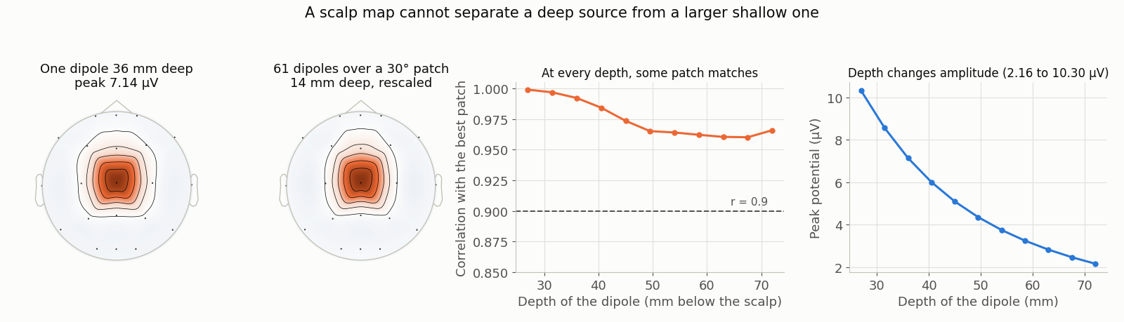
The figure is the argument in one picture. A deep dipole and a broad superficial patch produce the same scalp map to within a few percent, at every depth tested. That is not a resolution limitation to be improved with a better algorithm; the two configurations are nearly indistinguishable in the measurements, so no inverse method operating on those measurements can separate them. Depth changes amplitude, but so do source strength and source extent, so amplitude separates nothing on its own.

What follows is a working list, for expert review:

Defensible, with the method and its assumptions stated:

• A broad regional localization of a superficial cortical generator — lobar or gyral scale — when the point-spread width at that location has been computed and is smaller than the distinction being drawn.
• A relative claim within one study: this condition’s estimate is more anterior than that one’s, computed through one pipeline with one head model, where the systematic errors are shared and largely cancel.
• A difference in time course between two parcels whose separation exceeds the leakage between them (L5.6), when that leakage has been quantified rather than assumed away.
• A dipole fit where the one- or two-source assumption is independently motivated and the goodness of fit and confidence volume are reported.

Not defensible from scalp EEG alone:

• Any claim about a deep structure — hippocampus, amygdala, thalamus, brainstem. This is pf-deep-source-claims and it is the reason that pitfall exists. The scalp map of a deep source is reproducible by a superficial patch, the null space is large, and depth weighting is a choice that makes deep solutions appear, not a measurement that finds them.
• Sub-centimetre precision, or a claim resting on which of two adjacent gyri a maximum fell in.
• “The generator was here and nowhere else.” The estimate everywhere else is the point-spread function of the estimate here; a quiet map is not evidence of quiet cortex.
• A count of sources. Two sources can merge into one blob and one source can split into two; the number of maxima in a source map is a property of the method.
• Comparisons across studies with different montages, head models, priors or regularization. Those differences change the answer by more than most effects of interest.

What ships on this site, and what does not

No inverse solution ships with this lesson. Spec §6 asks for a dSPM of the P3 computed on ds-fsaverage, with a beamformer on the same data for comparison. That requires a template anatomy, and both candidate anatomies fail the site’s licence gate (L5.4): ds-fsaverage is governed by the FreeSurfer Software License Agreement, which permits derivative works only by propagating the whole agreement onto every copy, and ds-mne-sample’s licence is contested and is an open decision for the author. So there is no cortical surface, no source space built on one, and no precomputed source map anywhere in this level.

This is stated rather than worked around because the alternative — showing a picture and not saying where its anatomy came from — is the failure this whole level is about. What the lesson does instead is put the arithmetic where the picture would have been: the ill-posedness, the null space, the resolution matrix and the depth-versus-extent figure above are all computable with no anatomy at all, on a sphere model, and they carry the argument. The site already uses a sphere forward model in earnest elsewhere: the REST reference in L2.3 was computed with mne.make_sphere_model and a volume source space of 673 sources, with no MRI involved.

A learner who obtains fsaverage under FreeSurfer’s own terms can of course run the full comparison locally. What cannot happen is this site shipping the result.

The data behind this lesson

• The depth-versus-extent figure is synthetic: an analytic homogeneous-sphere forward model on the 21 10-20 electrode positions, average-referenced, no noise, generated by data/scripts/make_figures_p3.py. The figure is only produced if the featured depth matches at r ≥ 0.98 and every tested depth at r ≥ 0.9; otherwise it is skipped rather than shown weaker than described.
• ds-erpcore P3 is the data the lesson’s worked example would use. TODO(confirm): the author mirrors the ERP CORE entry into the catalogue registry and signs off the dataset page.
• ds-fsaverage is named in this lesson’s frontmatter because the lesson is about why it cannot be used here. No asset derived from it ships and no notebook downloads it.
• TODO(confirm): the localization error to expect from a template head model, from a given channel count, and from each inverse method is the central quantitative content of this lesson’s objectives, and this site has not sourced it. (Michel, 2019) is the reading-list entry; every number must come from there or from a primary source before publication.

Practice

The inverse problem on a sphere: the null space, minimum-norm, dSPM, sLORETA, eLORETA and an LCMV beamformer, resolution matrices, the depth bias — and why a deep source and a superficial patch cannot be told apart nb-5-5-inverse

Level 5 ~3 min

notebooks/L5/nb-5-5-inverse.ipynb

Open in Colab Download Read it here

The notebook works the inverse problem on a head model that needs no licensed anatomy: build a sphere forward model and a volume source space, form the minimum-norm, dSPM and LCMV operators from it, and then compute the resolution matrix for each — point-spread width and localization bias as a function of depth, and the cross-talk between a chosen pair of locations. Every claim in this lesson about depth bias, smoothing and resolution is a number you can produce that way. The dSPM-of-the-P3-on-fsaverage comparison §6 asks for is not run, for the licence reason above, and the notebook says so where that cell would have been.

Exercises

Exercise ex-5-5-which-claim

Multiple choice

Two source maps are computed from the same 32-channel ERP dataset with a template head model. Map A has its maximum on the lateral parietal surface; map B, from a different inverse method with different regularization, has its maximum in the hippocampus. Which claim can be defended, and on what grounds?

Options

The hippocampal claim, because the method that produced map B models deep sources explicitly and the other does notA cautious version of the lateral parietal claim: a superficial cortical generator at broad regional scale, with the method, head model, regularization and the computed point-spread width at that location all statedBoth, since the two maps come from the same data and each method has its own valid domainNeither: with 32 channels and a template head model no source claim of any kind is defensible

Check

Hint

Exercise ex-5-5-cannot-establish

Multiple select

Which of these does a linear EEG source estimate fail to establish, however good the fit to the sensor data? Select all that apply.

Options (select all that apply)

That the generator was in a deep structure rather than a broad superficial patchThat there were exactly two generators, because the map has two maximaThat the cortex outside the estimated region was inactiveThat one condition estimate is more anterior than the other, within the same study and pipelineThat the solution is the true source distribution, because it explains 99 % of the sensor variance

Check

Hint

Exercise ex-5-5-reporting

Free response

Write the methods-section paragraph for a source analysis: what must a reader be told before they can judge whether your localization claim is supported?

Your answer

Reveal model answer

Pitfalls

Pitfall

Overclaiming source depth or precision

Symptom

"Hippocampal generator" from 32 channels and a template head.

Cause

Two facts, and they compound.

Detect

• Ask what else would have produced the same scalp data. For a deep claim, the answer is always “a superficial patch”, and the figure below is the demonstration. If the analysis cannot exclude it, the claim is not supported. - Compute the point-spread function at the claimed location. It needs no data — only the inverse operator and the leadfield, Res = W·L — so there is never an excuse for not k…

Fix

• State the claim at the scale the resolution supports — lobar or broad regional, for a superficial cortical generator — and give the point-spread width at that location alongside it. - Prefer relative claims within one study. A difference between conditions computed through one pipeline shares its head-model, montage and prior errors between the two conditions, so much of the systematic error ca…

Full entry with example →

In other tools

In other toolsEEGLAB · FieldTrip — names only

The equivalents of what this lesson does, for a reader who works in another toolbox. Function names only: their own documentation is the place to learn how to call them.

EEGLAB

• pop_multifitdipfit plugin
• pop_dipplotdipfit plugin

FieldTrip

• ft_dipolefittingFieldTrip
• ft_sourceanalysisFieldTrip
• ft_sourceplotFieldTrip

Names checked 2026-09-18 against EEGLAB 2026.0.0 (plugins at the versions in EEGLAB’s own plugin list) and FieldTrip 20251218.

Reading

1. Michel & Brunet (2019). EEG source imaging practical review. unverified
2. Gramfort et al. (2014). MNE software. unverified