Clinical EEG primer (reading module)

Objectives

• Recognize what clinical review looks like (montages, activation procedures)
• Recognize the appearance of epileptiform discharges in published examples
• Explain why automated spike detection is hard
• State clearly what a research analyst must not claim

Why this matters

Sooner or later a research analyst opens a recording and sees something that looks wrong. What happens next is the subject of this module. Two things are worth knowing: enough about clinical review to recognise what you are looking at when you meet it — half of EEG’s vocabulary comes from the clinic — and, much more importantly, exactly where your competence stops and what you must not say when it does.

Concepts

How a clinical recording is actually read

A clinical EEG is not read in one view. The same recording is stepped through several montages, because the montage is the measurement (L0.2, L2.3) and each one answers a different question:

• a referential montage, every electrode against a common reference, which shows amplitude honestly and inherits whatever the reference is doing;
• a longitudinal bipolar montage — neighbouring electrodes chained front to back down each side, universally called the “double banana” — in which each trace is a difference between neighbours, so a trace is large only where the voltage changes between them;
• a transverse bipolar montage, the same idea across the head instead of along it.

The chains localise by phase reversal: in a bipolar chain a focal maximum shows up as two adjacent derivations deflecting in opposite directions, pointing at the electrode between them. That is the single most useful thing bipolar montages do, and it is why clinical readers switch montages rather than choosing one.

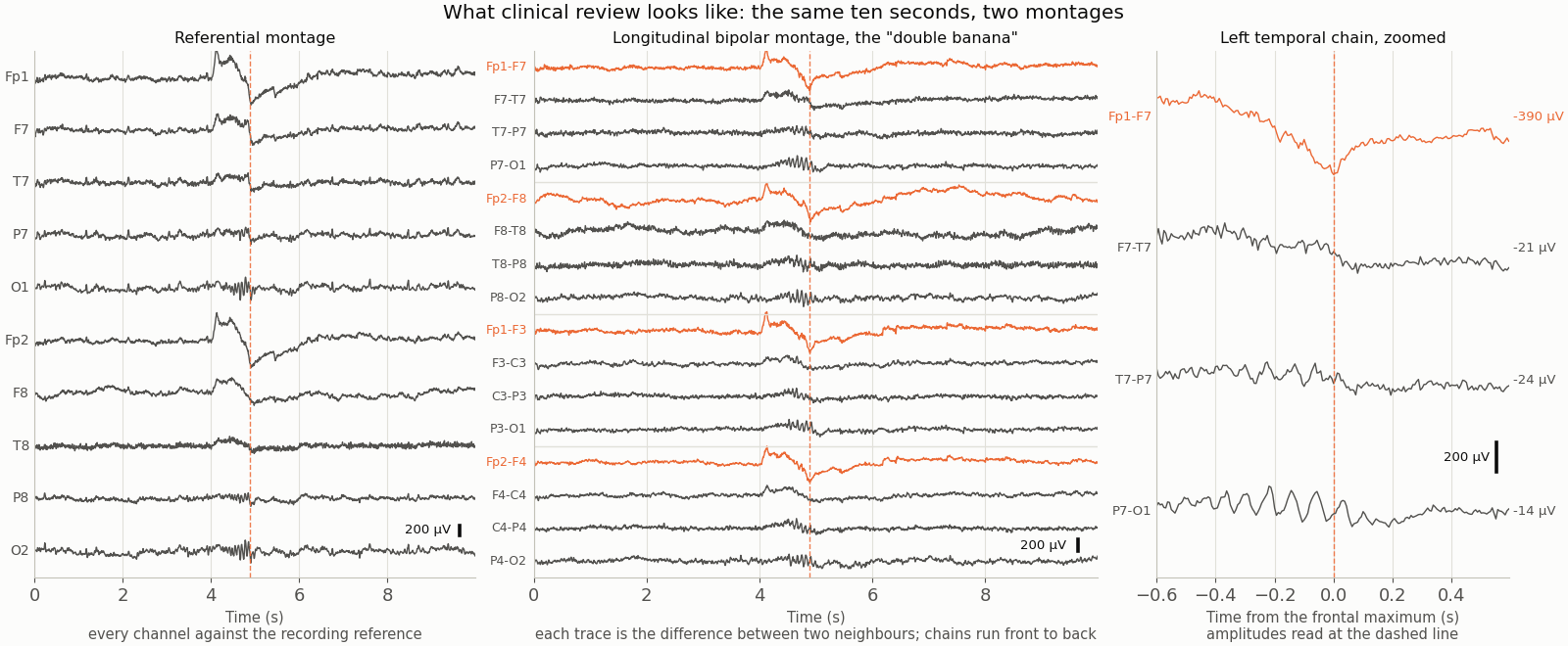
Alongside the montages, a clinical recording has a protocol rather than a paradigm: a period of quiet wakefulness with eyes opened and closed to command, and activation procedures intended to make abnormalities more likely to appear — hyperventilation, photic stimulation with a strobe at a series of flash rates, and drowsiness or sleep, sometimes after sleep deprivation. There are also technologist’s notes in the record: what the patient was doing, when they moved, when they were spoken to. In a clinical recording that log is part of the data, and its research equivalent — the event file — is usually much poorer.

TODO(confirm): the display conventions (paper speed, sensitivity in µV per millimetre, the standard filter settings a clinical review uses) and the durations and rates of the activation procedures are deliberately not quoted here. They are specified in professional guidelines that nobody on this project has read at a named edition, and a clinical parameter quoted from memory is exactly the kind of number this module is about not stating. (Kane et al., 2017) is the entry point for the vocabulary.

Epileptiform discharges: described here, shown elsewhere

The interictal findings a clinical reader is looking for are, in the field’s own terms, spikes, sharp waves and spike-and-wave complexes: transients that stand out from the background, have a particular morphology and a plausible physiological field, disrupt the ongoing activity, and are often followed by a slow wave. Whether something qualifies is a judgement about morphology in context — the background it interrupts, the state the patient is in, the field across the electrodes, whether it recurs in a consistent location — not a threshold crossing.

No figure of an epileptiform discharge appears on this site, and that is deliberate. Two reasons, and both are worth stating plainly rather than leaving as an absence:

• No dataset in this site’s directory whose licence permits shipping derived assets contains scored epileptiform activity. The asset track checked and recorded it; there is nothing honest to crop.
• Simulating one would fabricate exactly the thing this module warns against. A plausible-looking drawn spike would teach people to recognise a shape that a script invented, in a module whose entire argument is that morphology in context is a clinical judgement. The site would be manufacturing a clinical finding in order to caution against over-reading clinical findings.

So the objective “recognise the appearance of epileptiform discharges in published examples” is served by published examples: the clinical literature, the atlases, and the figures in the guidelines that define the terms. Go and look at them there, in a source that took responsibility for the label, with the patient context and the montage that the label depended on. A cropped, unlabelled waveform on a teaching site is worse than nothing, because it looks like enough.

Why automated spike detection is hard

Four reasons, and only the first is about signal processing.

The ground truth disagrees with itself. Expert readers do not perfectly agree on which transients are epileptiform, so the labels a detector is trained and scored against are a reader’s judgement, and a detector that matches one reader may disagree with another. Any reported sensitivity is sensitivity against a particular labelling.

The events are rare and the recording is long. This is the constraint that defeats most detectors, and it is arithmetic rather than neuroscience. Take a 20-minute routine recording scanned in one-second windows — 1200 windows — containing five discharges. A detector with 95 % sensitivity and 99 % specificity finds about 4.75 of the five, and raises about 12 false alarms from the 1195 windows that contain nothing. Fewer than three in ten of its alarms are real, at a specificity that sounds excellent. Lengthen the recording to a day of monitoring and the false alarms scale with the hours while the events do not.

Everything else in the record has transients too. Electrode pops, movement, muscle, ECG and eye movements all produce sharp, high-amplitude, short-lived deflections, and most of them are more common than the target.

Detectors do not transport. A detector tuned on one montage, one amplifier, one filter chain and one patient population meets a different one and its operating point moves. This is pf-site-device-confound in a clinical costume.

Artifacts that mimic pathology

Three failure modes, ranked by how often a research analyst will actually meet them:

Eye movements read as focal frontal events. The figure above is the demonstration: a blink is a large, focal, frontally maximal transient with a phase reversal at the top of the chain, and so is a frontal discharge. What separates them is the field (a blink is symmetric, vertical, with its maximum at Fp1/Fp2 and no cortical field below), the morphology, the accompanying EOG, and physiological plausibility. A lateral eye movement gives opposite-polarity deflections at F7 and F8, which looks striking and is not a finding.

Muscle read as fast pathology. Scalp muscle produces spiky, broadband, high-frequency activity concentrated at the lateral rim — the same electrodes where temporal discharges are looked for.

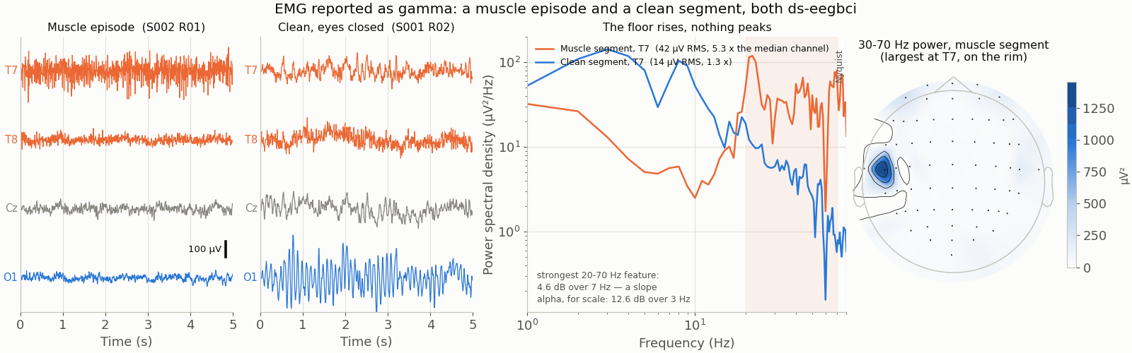
Electrode artifacts read as focal transients. A single electrode popping produces a sharp deflection in one channel with no field at its neighbours, which is exactly the thing a bipolar chain is good at exposing: a real cortical event has a field, an electrode event does not.

The research analyst’s version of all three is the same discipline L0.5 teaches: look at the field across the head and at the other channels before you interpret a waveform on one.

What a research analyst must not claim

This is the section that matters, and it is the one to reread. All of the following are outside the competence this site provides, and a research analyst writing them has made a clinical claim:

• That a recording, or anything in it, is normal or abnormal. “Normal EEG” is a clinical conclusion. The absence of anything you noticed is not evidence of normality; you are not screening.
• That a transient is epileptiform, a spike, a sharp wave, or “epileptiform-like”. The hedged version is not safer — it is the same claim with deniability.
• That a participant has, or does not have, any condition, or that a finding is consistent with one. This includes the softer forms: “suggestive of”, “compatible with”, “worth investigating”.
• That an incidental finding requires action, or that it does not. The judgement about what an unexpected feature means belongs to a clinician; the analyst’s job is the referral, not the triage.
• That a device, an index or a pipeline detects, screens for, monitors or assesses a clinical condition. Those verbs have a regulatory meaning, and applying them to a research measure is a claim about a medical device.
• That a group difference in an EEG measure between a patient group and controls is a biomarker, a diagnostic or a marker of anything. A significant group difference is a group difference; L7.6 is the lesson about the distance between that and a biomarker, and it is long.

Two obligations that go with the prohibitions, because a list of things not to say is not a protocol:

Have an incidental-findings procedure before you record. Who looks, on what timescale, what is told to the participant, and what the consent form promised. Deciding this after you have seen something is too late, and “we will deal with it if it happens” is not a procedure. Most ethics frameworks require one; TODO(confirm): the specific requirements vary by jurisdiction and institution and none has been read for this module.

Describe what you measured, not what it means. “A high-amplitude frontally maximal transient occurred at 00:04:12” is a description anybody can check. Everything beyond it is somebody else’s professional judgement, and the discipline of stopping at the description is the same one the rest of this level teaches about every other kind of claim.

Explore

This module has no widget. The activity is reading, and it has three parts:

• Work the figure above without its caption. Cover the text, find the frontal maximum in the referential panel, then trace it down the bipolar chains and predict which link carries it. Then read the caption and notice that the correct identification was available from the field and the symmetry, not from the waveform’s shape.
• Go and look at published discharges, in an atlas or in the figures accompanying the standard glossary ( (Kane et al., 2017) ), with the patient context and the montage the label depended on. Notice how much of the label rests on things a cropped waveform does not carry.
• Then go back to the artifact drill. The Spot the artifact lab from L0.5 is the closest this site comes to the discrimination this module is about, and it is a drill on artifacts — which is exactly the half of the problem a research analyst is competent to do.

Practice

This module has no notebook, and nothing computational to run. That is not an omission: there is no dataset here to compute on, because the module’s examples are published figures rather than this site’s data, and the only executable version of “recognise a discharge” would require a labelled discharge that no licence-clear dataset in the directory provides.

The practice is a written one. Take a recording you have analysed and write two paragraphs: what you observed, in descriptive terms only; and what you would do if you saw something you did not expect, naming the person who would look at it and the timescale. If your project has no answer to the second paragraph, that is the finding.

Exercises

Exercise ex-7-4-scope-scenario

Multiple choice

You are the analyst on a healthy-volunteer resting-state study. Preprocessing one participant's recording, you notice a repeated sharp transient over the left temporal electrodes that does not look like any artifact you recognise. What is the appropriate next step?

Options

Note it in the QC report as a probable epileptiform discharge, exclude the participant, and move on.Follow the study’s incidental-findings procedure: describe what you observed without interpreting it, and route it to the clinically qualified person the protocol names, on the timescale it states.Run an automated spike detector; if it fires, the finding is confirmed and the participant should be informed.Do nothing. The study is not clinical, the participant was screened as healthy, and interpreting the recording is outside your competence.

Check

Hint

Exercise ex-7-4-must-not-claim

Multiple select

Your group has found that a resting-state EEG measure differs significantly between a patient sample and matched controls. Select every statement that a research analyst may NOT make on the strength of that result.

Options (select all that apply)

The measure differed between the two groups, with this effect size and this confidence interval.The measure is a biomarker for the condition.The measure can be used to screen for the condition.Individual recordings in the patient group frequently showed the pattern, though the group distributions overlap substantially.A recording with a high value on this measure is suggestive of the condition.The group difference is consistent with the condition and warrants clinical investigation in individuals.

Check

Hint

Exercise ex-7-4-detector-precision

Numeric

A spike detector scans a 20-minute recording in one-second windows (1200 windows) containing 5 discharges. It has 95 % sensitivity and 99 % specificity. Of the alarms it raises, what percentage are real discharges, to one decimal place?

Your answer %

Accepted within ±0.5 %.

Check

Hint

Pitfalls

In other tools

Neither EEGLAB nor FieldTrip has an equivalent, and that is the honest answer rather than a gap. This module is about montages a clinical reader steps through, procedures a technologist runs, a body of published examples, and the boundary of a professional competence. None of that is a function call, in either toolbox or in any other. The montage conventions the module describes are constructed in both tools with their ordinary re-referencing machinery — the same functions L2.3 already names — and nothing here would be clarified by repeating them. Verified by the site’s own survey of both toolboxes at named releases, recorded in site/src/lib/site/other-tools.ts; several lessons on Levels 0–6 leave this sidebar empty for the same reason.

Reading

1. Kane et al. (2017). Revised glossary of clinical EEG terms. unverified